MATH 3850: Numerical Optimization

Adam: A Method for
Stochastic Optimization

Reproducing key results from Kingma & Ba (ICLR 2015)

Gurman Basran & Qusai Quresh
University of Lethbridge, Winter 2026
April 2, 2026

5 optimizers implemented from scratch in NumPy · 5 experiments · PyTorch validation

Part 1: Explaining the Algorithm

The Problem: Why Not Just Use Gradient Descent?

Two problems we ran into in class, and what motivated Adam

Problem 1: One Step-Size for All

In gradient descent, we use a single $\alpha$ for every parameter. If the landscape is stretched out in one direction (high $\kappa$), GD zigzags back and forth across the narrow direction and barely makes progress along the wide direction.

From class (Theorem 3.4): the convergence rate of steepest descent is $\frac{\kappa - 1}{\kappa + 1}$. If $\kappa = 2500$, thats $\frac{2499}{2501} \approx 0.999$, meaning each step only reduces the error by 0.1%.

Problem 2: Noisy Gradients

In machine learning we dont compute the gradient on ALL the data. We use a small random minibatch (128 samples out of 60,000), so $g_t$ is noisy. That makes the zigzag even worse.

Methods like Newtons method and BFGS from class dont work here because they need exact gradients and store an $n \times n$ matrix ($O(n^2)$ memory), which is impossible with millions of parameters.

Part 1: Explaining the Algorithm

The Idea: Combine Two Ingredients

Adam = Momentum + Adaptive Learning Rates + Bias Correction

Ingredient 1: Momentum

Keep a running average of the gradient direction. Smooths out noise so you move steadily.

$$m_t = \beta_1 \cdot m_{t-1} + (1 - \beta_1) \cdot g_t$$

$m_t$: momentum estimate (first moment); smoothed gradient direction
$\beta_1$: momentum decay rate; typically 0.9 (keep 90% of old, mix in 10% new)
$g_t$: gradient at the current timestep

Ingredient 2: Adaptive Rates

Track how volatile each parameter is. Big gradients get smaller steps; small gradients get bigger steps.

$$v_t = \beta_2 \cdot v_{t-1} + (1 - \beta_2) \cdot g_t^2$$

$v_t$: scale estimate (second moment); tracks gradient magnitude per parameter
$\beta_2$: scale decay rate; typically 0.999 (very slow-moving average)
$g_t^2$: element-wise squared gradient

Bias correction: Both $m_t$ and $v_t$ start at zero, so early estimates are too small. Adam corrects this: $\hat{m}_t = m_t \,/\, (1 - \beta_1^t)$ and $\hat{v}_t = v_t \,/\, (1 - \beta_2^t)$. The correction vanishes as $t$ grows large.

Part 1: Explaining the Algorithm

Algorithm 1: Adam (from the paper)

Kingma & Ba (2015), page 2. Every line explained.

Initialization

1 $m_0 \leftarrow 0$, $v_0 \leftarrow 0$, $t \leftarrow 0$ all zeros to start

Repeat Until Converged

2 $t \leftarrow t + 1$ bump the clock

3 $g_t \leftarrow \nabla f_t(\theta_{t-1})$ gradient on minibatch

4 $m_t \leftarrow \beta_1 \cdot m_{t-1} + (1 - \beta_1) \cdot g_t$ update momentum

5 $v_t \leftarrow \beta_2 \cdot v_{t-1} + (1 - \beta_2) \cdot g_t^2$ update scale

6 $\hat{m}_t \leftarrow m_t \,/\, (1 - \beta_1^t)$ correct momentum bias

7 $\hat{v}_t \leftarrow v_t \,/\, (1 - \beta_2^t)$ correct scale bias

8 $\theta_t \leftarrow \theta_{t-1} - \alpha \cdot \hat{m}_t \,/\, (\sqrt{\hat{v}_t} + \epsilon)$ THE UPDATE

Hyperparameters

$\alpha$: step-size (learning rate). Default: 0.001
$\beta_1$: momentum decay. Default: 0.9
$\beta_2$: scale decay. Default: 0.999
$\epsilon$: numerical safety. Default: $10^{-8}$

Why This Works

Line 8 is the key: $\hat{m}_t$ tells us the direction. $\sqrt{\hat{v}_t}$ normalizes by magnitude. The ratio $\hat{m}_t / \sqrt{\hat{v}_t}$ gives each parameter its own effective step size. The paper shows each step is approximately bounded by $\alpha$, which is the trust region property.

Part 1: Explaining the Algorithm

Data Flow: How the Pieces Connect

The gradient splits into two paths, then recombines for the update

The Key Insight

The gradient gets split into two separate streams of information: $\hat{m}_t$ captures the direction to go, and $\sqrt{\hat{v}_t}$ captures the magnitude to normalize by. When we divide direction by magnitude, each parameter gets its own appropriately-sized step. This is analogous to what BFGS does with the inverse Hessian $H_k^{-1}$, but Adam does it with just $O(n)$ memory instead of $O(n^2)$.

Part 2: Code Demonstration

From Paper to NumPy: Our Implementation

Algorithm 1 translated line-by-line into Python

Adam Optimizer Class (from our notebook)

class Adam:
    def __init__(self, lr=0.001, beta1=0.9, beta2=0.999, eps=1e-8):
        self.lr    = lr     # alpha (step-size)
        self.beta1 = beta1  # beta_1 (momentum decay)
        self.beta2 = beta2  # beta_2 (scale decay)
        self.eps   = eps    # epsilon (safety)
        self.m = None       # m_t (first moment)
        self.v = None       # v_t (second moment)
        self.t = 0          # timestep counter

    def step(self, params, grads):
        self.t += 1                                  # line 2
        self.m = self.beta1 * self.m \
              + (1 - self.beta1) * grads              # line 4
        self.v = self.beta2 * self.v \
              + (1 - self.beta2) * grads ** 2         # line 5
        m_hat = self.m / (1 - self.beta1 ** self.t)  # line 6
        v_hat = self.v / (1 - self.beta2 ** self.t)  # line 7
        return params - self.lr * m_hat \
             / (np.sqrt(v_hat) + self.eps)            # line 8

Training Loop

for epoch in range(n_epochs):
    for X_batch, y_batch in get_minibatches(
            X_train, y_train, batch_size=128):
        dW, db, loss = compute_gradients(
            X_batch, y_batch, W, b)
        grads = flatten_params(dW, db)
        params = optimizer.step(params, grads)

Model: Softmax + Cross-Entropy Gradient

def compute_gradients(X, y_true, W, b):
    y_pred = softmax(X @ W + b)
    dZ = y_pred - y_true
    dW = X.T @ dZ / batch_size   # clean matrix form
    db = np.mean(dZ, axis=0)
    loss = cross_entropy_loss(y_pred, y_true)
    return dW, db, loss

Line-by-line match: Each comment on the left maps directly to a line number in Algorithm 1. The only difference is NumPy vectorization: all 7,850 parameters update simultaneously in one array operation.

Part 3: Experiments

Experiment 1: MNIST Logistic Regression

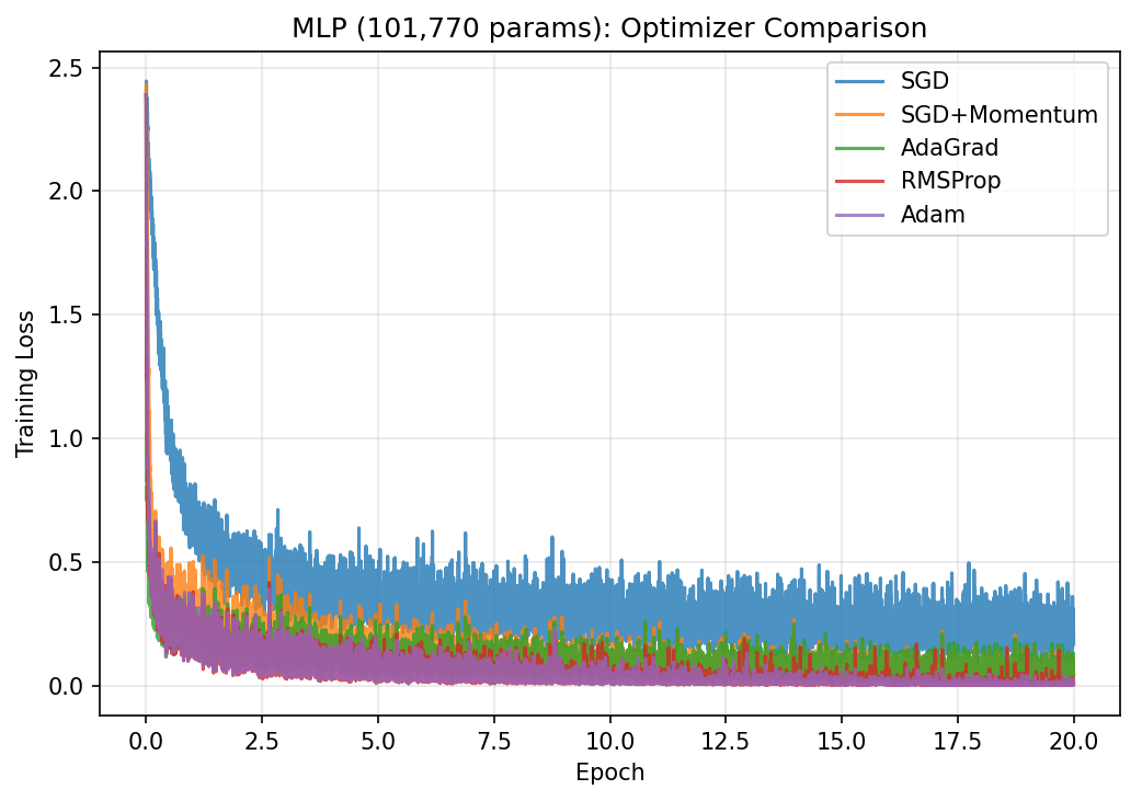
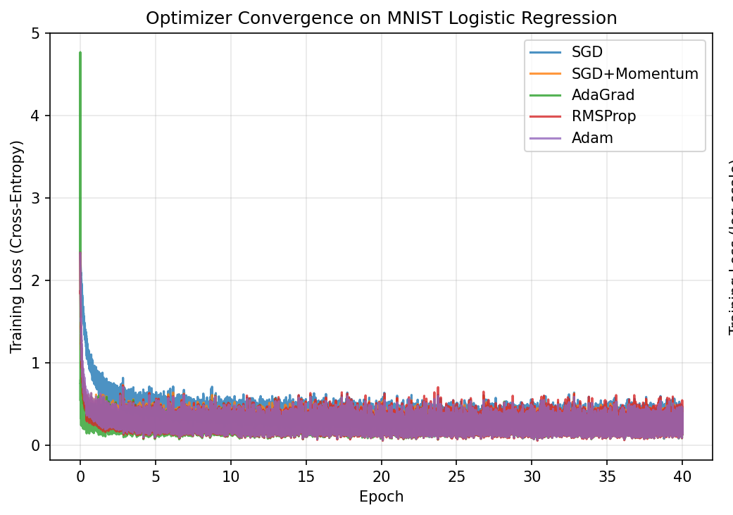
Reproducing Section 6.1 of the paper: 5 optimizers, 40 epochs, same starting weights

Training loss vs epoch (linear scale)

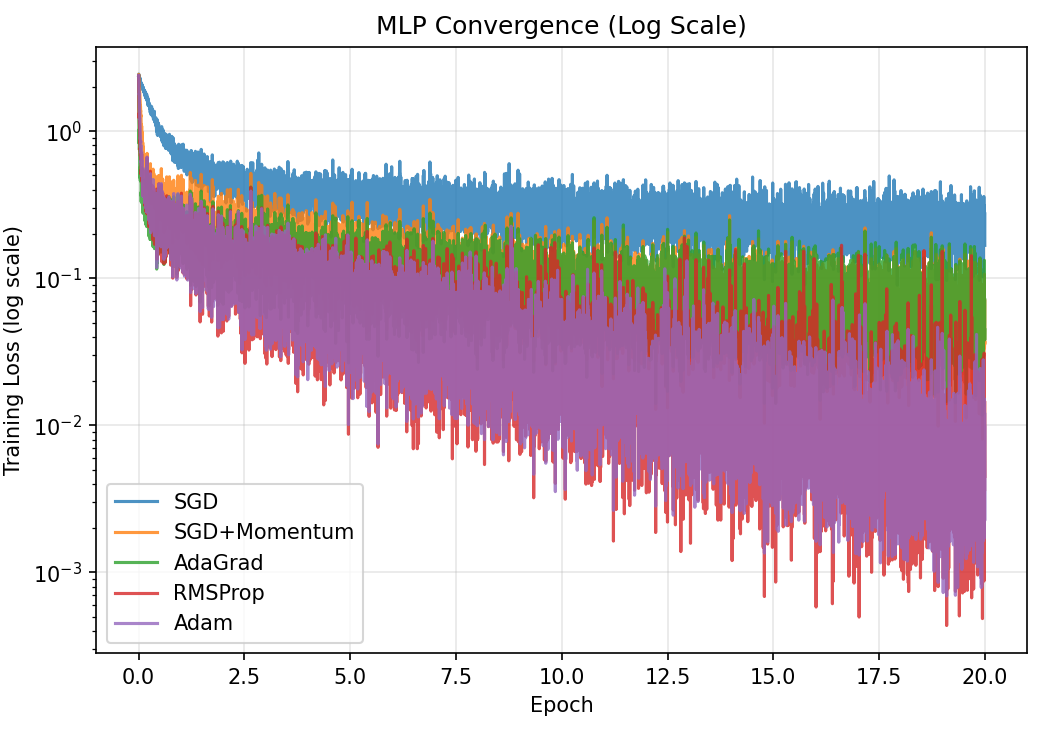
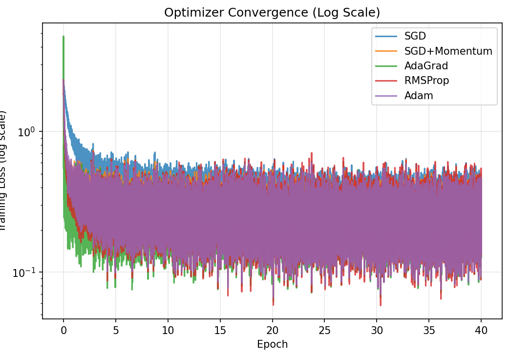
Training loss vs epoch (log scale; stretches out differences at the bottom)

Setup: 60,000 MNIST images (28x28 pixels, 784 features), 10 digit classes. Minibatch size 128. All 5 optimizers start from the same random initial weights. Logistic regression: $\hat{y} = \text{softmax}(XW + b)$, cross-entropy loss. Total: 7,850 parameters.

Optimizer	Test Accuracy	Final Loss
SGD	91.58%	0.321
SGD + Momentum	92.36%	0.274
AdaGrad	92.72%	0.264
RMSProp	92.65%	0.260
Adam	92.69%	0.258

Key Finding

All adaptive methods beat plain SGD, consistent with the papers trends. The differences between Adam, AdaGrad, and RMSProp are small here because logistic regression is a convex problem. Adam and Momentum converge fastest in the early epochs.

Part 3: Experiments

Experiment 2: Is Our Code Correct?

Validating our from-scratch Adam against PyTorchs torch.optim.Adam

Full run: 4,690 iterations. Both lines overlap perfectly.

Zoomed: first 500 iterations. Still indistinguishable.

Setup: Run our Adam and PyTorchs torch.optim.Adam on identical data, same initial weights, same batch ordering, same hyperparameters ($\alpha = 0.001$, $\beta_1 = 0.9$, $\beta_2 = 0.999$). Compare loss values at every single iteration.

Why: Before we trust any of our other experimental results, we need to prove that we actually implemented Algorithm 1 correctly. We checked PyTorchs source code on GitHub (torch/optim/adam.py) to confirm they implement the same version of the algorithm.

Result

Over 4,690 iterations (10 epochs × 469 batches):
Max absolute loss difference = $6.34 \times 10^{-7}$

The tiny difference comes from floating-point rounding between NumPy and PyTorch, not from an error in our code.

Part 3: Experiments

Experiment 3: Rosenbrock Function

Connecting to our coursework: the same test function from textbook Chapter 3

Contour map with optimizer paths. Start: $(-1, 1)$. Target: $(1, 1)$.

Function value vs iteration (lower is better; $f = 0$ at minimum).

$$f(x,y) = (1-x)^2 + 100(y-x^2)^2$$

Long narrow curved valley. $\kappa \approx 2500$ near minimum.

Why we added this: This experiment is NOT from the Adam paper. We included it to connect back to our coursework. Adam was designed for stochastic optimization (noisy minibatch gradients), not deterministic functions where you have the exact gradient.

Optimizer	Final $f$ value
SGD	1.47
SGD + Momentum	0.00007
AdaGrad	0.000002
RMSProp	0.15
Adam	0.043

Key Finding

Momentum and AdaGrad beat Adam here. Makes sense: Adam was built for noisy gradients, and Rosenbrock gives exact gradients. Plain SGD barely moved (f=1.47), matching the class prediction that steepest descent struggles when $\kappa \approx 2500$ because $(\kappa-1)/(\kappa+1) \approx 0.999$.

Part 3: Experiments

Experiment 4: Hyperparameter Sensitivity

Section 6.4 of the paper: which settings matter most?

Varying $\alpha$: curves spread far apart. HIGH impact.

Varying $\beta_1$: tight cluster. Low impact.

Varying $\beta_2$: tight cluster. Low impact.

Setup: Vary $\alpha$, $\beta_1$, and $\beta_2$ one at a time while keeping the others at their paper defaults. Train logistic regression on MNIST for 20 epochs.

What We Found

Parameter	Range Tested	Loss Range	Impact
$\alpha$	0.0001 to 0.005	0.209 to 0.267	HIGH
$\beta_1$ (momentum)	0.0 to 0.99	0.210 to 0.215	LOW
$\beta_2$ (scale)	0.9 to 0.9999	0.215 to 0.223	LOW

Key Finding

$\alpha$ is the one that matters. The $\beta$ values are robust across a wide range, just like the paper claims (Section 6.4). Best result: $\alpha = 0.005$ gave the lowest final loss of 0.209. This is good news: you really only have to tune one hyperparameter.

Part 3: Experiments

Experiment 5: Neural Network (MLP) on MNIST

Section 6.2 of the paper: where Adam really shines

MLP training loss vs epoch (linear scale). Adam drops fastest.

Log scale: Adam and RMSProp clearly separate from SGD.

Setup: 784 → 128 (ReLU) → 10 (softmax). Backprop from scratch. He init. 20 epochs, batch 128. Non-convex, 101,770 params (13x logistic).

Optimizer	Test Accuracy	Gap vs SGD
SGD	93.80%
SGD + Momentum	97.72%	+3.92
AdaGrad	97.34%	+3.54
RMSProp	97.92%	+4.12
Adam	97.97%	+4.17

Key Finding

Adam 97.97% vs SGD 93.80% (4+ point gap). Much larger than the ~1 point gap on logistic regression. RMSProp close at 97.92% (Adam = RMSProp + momentum + bias correction). Non-convex + more params = adaptive step sizes matter.

Wrap-Up

How Adam Connects to This Course

The evolution of step-size strategies we studied in MATH 3850

Gradient Descent

Nocedal & Wright, Chapter 3

$$x_{k+1} = x_k - \alpha \nabla f(x_k)$$

Step-size: One $\alpha$ (step-size) for everything, or found via line search
Curvature: Ignores curvature entirely
Memory: $O(n)$

BFGS

Nocedal & Wright, Chapter 6

$$x_{k+1} = x_k - \alpha_k H_k^{-1} \nabla f(x_k)$$

Step-size: $H_k^{-1}$ (inverse Hessian approximation) scales the gradient
Curvature: Full $n \times n$ matrix of curvature info
Memory: $O(n^2)$

Adam

Kingma & Ba, 2015

$$\theta_t = \theta_{t-1} - \alpha \frac{\hat{m}_t}{\sqrt{\hat{v}_t} + \epsilon}$$

Step-size: $\hat{m}_t / \sqrt{\hat{v}_t}$ gives per-parameter adaptive scaling
Curvature: Diagonal approximation from gradient history
Memory: $O(n)$

The Deep Connection

All three methods are doing the same thing: using gradient history to take smarter steps. GD uses just the raw gradient. BFGS builds a full curvature matrix for perfect scaling but needs $O(n^2)$ memory. Adam takes the same concept of "scale the gradient smartly" but uses a diagonal approximation ($\hat{m}_t / \sqrt{\hat{v}_t}$) that only needs $O(n)$ memory. Its like a practical compromise between the simplicity of GD and the intelligence of BFGS, designed for the noisy, high-dimensional world of machine learning.

Summary

What we found across five experiments

1. All adaptive methods beat plain SGD on MNIST, matching the papers trends (Section 6.1).

2. Our implementation is correct: max diff vs PyTorch = $6.34 \times 10^{-7}$ over 4,690 iterations.

3. Adam struggles on deterministic problems (Rosenbrock), confirming it was built for noisy gradients.

4. $\alpha$ is the only hyperparameter that really matters. $\beta_1$ and $\beta_2$ are robust.

5. Adam shines on non-convex problems: 97.97% on MLP vs 93.80% SGD (4+ point gap).

References: Kingma & Ba (2015), "Adam: A Method for Stochastic Optimization," ICLR. · Ruder (2016), "An overview of gradient descent optimization algorithms." · Nocedal & Wright, Numerical Optimization, 2nd ed.

Adam: A Method forStochastic Optimization

The Problem: Why Not Just Use Gradient Descent?

Problem 1: One Step-Size for All

Problem 2: Noisy Gradients

The Idea: Combine Two Ingredients

Ingredient 1: Momentum

Ingredient 2: Adaptive Rates

Algorithm 1: Adam (from the paper)

Hyperparameters

Why This Works

Data Flow: How the Pieces Connect

The Key Insight

From Paper to NumPy: Our Implementation

Experiment 1: MNIST Logistic Regression

Key Finding

Experiment 2: Is Our Code Correct?

Result

Experiment 3: Rosenbrock Function

Key Finding

Experiment 4: Hyperparameter Sensitivity

What We Found

Key Finding

Experiment 5: Neural Network (MLP) on MNIST

Key Finding

How Adam Connects to This Course

Gradient Descent

BFGS

Adam

The Deep Connection

Summary

Questions?

Adam: A Method for
Stochastic Optimization